4  Hướng dẫn vẽ đồ thị nhiều trục Y

Nguyên tắc chung khi vẽ nhiều trục Y hay X là ta sẽ set par(new = TRUE) để tạo ra 1 plot mới dán đè lên plot hiện tại với scale trục Y mới, ta thay đổi vị trí các trục Y bằng lệnh axis().

4.1 Tham khảo

https://evolvingspaces.blogspot.com/2011/05/multiple-y-axis-in-r-plot.html

#Create Dataset

time<-seq(7000,3400,-200)
pop<-c(200,400,450,500,300,100,400,700,830,1200,400,350,200,700,370,800,200,100,120)
grp<-c(2,5,8,3,2,2,4,7,9,4,4,2,2,7,5,12,5,4,4)
med<-c(1.2,1.3,1.2,0.9,2.1,1.4,2.9,3.4,2.1,1.1,1.2,1.5,1.2,0.9,0.5,3.3,2.2,1.1,1.2)

#Define Margins. The trick is to use give as much space possible on the left margin (second value)
par(mar=c(5, 12, 4, 4) + 0.1)

#Plot the first time series. Notice that you don't have to draw the axis nor the labels

plot(time, pop, axes=F, ylim=c(0,max(pop)), xlab="", ylab="",type="l",col="black", main="",xlim=c(7000,3400))
points(time,pop,pch=20,col="black")
axis(2, ylim=c(0,max(pop)),col="black",lwd=2)
mtext(2,text="Population",line=2)

#Plot the second time series. The command par(new=T) is handy here. 
#If you just need to plot two timeseries, you could also use the right vertical axis as well. 
#In that case you have to substitute "2" with "4" in the functions axis() and mtext(). 
#Notice that in both functions lines is increased so that the new axis and 
#its label is placed to the left of the first one. 
#You don't need to increase the value if you use the right vertical axis.

par(new=T)
plot(time, med, axes=F, ylim=c(0,max(med)), xlab="", ylab="", 
type="l",lty=2, main="",xlim=c(7000,3400),lwd=2)
axis(2, ylim=c(0,max(med)),lwd=2,line=3.5)
points(time, med,pch=20)
mtext(2,text="Median Group Size",line=5.5)

#Plot the third time series. Again the line parameter are both further increased.

par(new=T)
plot(time, grp, axes=F, ylim=c(0,max(grp)), xlab="", ylab="", 
type="l",lty=3, main="",xlim=c(7000,3400),lwd=2)
axis(2, ylim=c(0,max(grp)),lwd=2,line=7)

points(time, grp,pch=20)
mtext(2,text="Number of Groups",line=9)

#We can now draw the X-axis, which is of course shared by all the three time-series.

axis(1,pretty(range(time),10))
mtext("cal BP",side=1,col="black",line=2)

#And then plot the legend.

legend(x=7000,y=12,legend=c("Population","Median Group Size","Number of Groups"),lty=c(1,2,3))

4.2 Vẽ đồ thị nhiều trục Y

Sử dụng dataset airquality. Daily readings of the following air quality values for May 1, 1973 (a Tuesday) to September 30, 1973.

• Ozone: Mean ozone in parts per billion from 1300 to 1500 hours at Roosevelt Island

• Solar.R: Solar radiation in Langleys in the frequency band 4000–7700 Angstroms from 0800 to 1200 hours at Central Park

• Wind: Average wind speed in miles per hour at 0700 and 1000 hours at LaGuardia Airport

• Temp: Maximum daily temperature in degrees Fahrenheit at La Guardia Airport.

A data frame with 153 observations on 6 variables.

[,1] Ozone numeric Ozone (ppb)

[,2] Solar.R numeric Solar R (lang)

[,3] Wind numeric Wind (mph)

[,4] Temp numeric Temperature (degrees F)

[,5] Month numeric Month (1–12)

[,6] Day numeric Day of month (1–31)

Source: The data were obtained from the New York State Department of Conservation (ozone data) and the National Weather Service (meteorological data).

airquality

    Ozone Solar.R Wind Temp Month Day
1      41     190  7.4   67     5   1
2      36     118  8.0   72     5   2
3      12     149 12.6   74     5   3
4      18     313 11.5   62     5   4
5      NA      NA 14.3   56     5   5
6      28      NA 14.9   66     5   6
7      23     299  8.6   65     5   7
8      19      99 13.8   59     5   8
9       8      19 20.1   61     5   9
10     NA     194  8.6   69     5  10
11      7      NA  6.9   74     5  11
12     16     256  9.7   69     5  12
13     11     290  9.2   66     5  13
14     14     274 10.9   68     5  14
15     18      65 13.2   58     5  15
16     14     334 11.5   64     5  16
17     34     307 12.0   66     5  17
18      6      78 18.4   57     5  18
19     30     322 11.5   68     5  19
20     11      44  9.7   62     5  20
21      1       8  9.7   59     5  21
22     11     320 16.6   73     5  22
23      4      25  9.7   61     5  23
24     32      92 12.0   61     5  24
25     NA      66 16.6   57     5  25
26     NA     266 14.9   58     5  26
27     NA      NA  8.0   57     5  27
28     23      13 12.0   67     5  28
29     45     252 14.9   81     5  29
30    115     223  5.7   79     5  30
31     37     279  7.4   76     5  31
32     NA     286  8.6   78     6   1
33     NA     287  9.7   74     6   2
34     NA     242 16.1   67     6   3
35     NA     186  9.2   84     6   4
36     NA     220  8.6   85     6   5
37     NA     264 14.3   79     6   6
38     29     127  9.7   82     6   7
39     NA     273  6.9   87     6   8
40     71     291 13.8   90     6   9
41     39     323 11.5   87     6  10
42     NA     259 10.9   93     6  11
43     NA     250  9.2   92     6  12
44     23     148  8.0   82     6  13
45     NA     332 13.8   80     6  14
46     NA     322 11.5   79     6  15
47     21     191 14.9   77     6  16
48     37     284 20.7   72     6  17
49     20      37  9.2   65     6  18
50     12     120 11.5   73     6  19
51     13     137 10.3   76     6  20
52     NA     150  6.3   77     6  21
53     NA      59  1.7   76     6  22
54     NA      91  4.6   76     6  23
55     NA     250  6.3   76     6  24
56     NA     135  8.0   75     6  25
57     NA     127  8.0   78     6  26
58     NA      47 10.3   73     6  27
59     NA      98 11.5   80     6  28
60     NA      31 14.9   77     6  29
61     NA     138  8.0   83     6  30
62    135     269  4.1   84     7   1
63     49     248  9.2   85     7   2
64     32     236  9.2   81     7   3
65     NA     101 10.9   84     7   4
66     64     175  4.6   83     7   5
67     40     314 10.9   83     7   6
68     77     276  5.1   88     7   7
69     97     267  6.3   92     7   8
70     97     272  5.7   92     7   9
71     85     175  7.4   89     7  10
72     NA     139  8.6   82     7  11
73     10     264 14.3   73     7  12
74     27     175 14.9   81     7  13
75     NA     291 14.9   91     7  14
76      7      48 14.3   80     7  15
77     48     260  6.9   81     7  16
78     35     274 10.3   82     7  17
79     61     285  6.3   84     7  18
80     79     187  5.1   87     7  19
81     63     220 11.5   85     7  20
82     16       7  6.9   74     7  21
83     NA     258  9.7   81     7  22
84     NA     295 11.5   82     7  23
85     80     294  8.6   86     7  24
86    108     223  8.0   85     7  25
87     20      81  8.6   82     7  26
88     52      82 12.0   86     7  27
89     82     213  7.4   88     7  28
90     50     275  7.4   86     7  29
91     64     253  7.4   83     7  30
92     59     254  9.2   81     7  31
93     39      83  6.9   81     8   1
94      9      24 13.8   81     8   2
95     16      77  7.4   82     8   3
96     78      NA  6.9   86     8   4
97     35      NA  7.4   85     8   5
98     66      NA  4.6   87     8   6
99    122     255  4.0   89     8   7
100    89     229 10.3   90     8   8
101   110     207  8.0   90     8   9
102    NA     222  8.6   92     8  10
103    NA     137 11.5   86     8  11
104    44     192 11.5   86     8  12
105    28     273 11.5   82     8  13
106    65     157  9.7   80     8  14
107    NA      64 11.5   79     8  15
108    22      71 10.3   77     8  16
109    59      51  6.3   79     8  17
110    23     115  7.4   76     8  18
111    31     244 10.9   78     8  19
112    44     190 10.3   78     8  20
113    21     259 15.5   77     8  21
114     9      36 14.3   72     8  22
115    NA     255 12.6   75     8  23
116    45     212  9.7   79     8  24
117   168     238  3.4   81     8  25
118    73     215  8.0   86     8  26
119    NA     153  5.7   88     8  27
120    76     203  9.7   97     8  28
121   118     225  2.3   94     8  29
122    84     237  6.3   96     8  30
123    85     188  6.3   94     8  31
124    96     167  6.9   91     9   1
125    78     197  5.1   92     9   2
126    73     183  2.8   93     9   3
127    91     189  4.6   93     9   4
128    47      95  7.4   87     9   5
129    32      92 15.5   84     9   6
130    20     252 10.9   80     9   7
131    23     220 10.3   78     9   8
132    21     230 10.9   75     9   9
133    24     259  9.7   73     9  10
134    44     236 14.9   81     9  11
135    21     259 15.5   76     9  12
136    28     238  6.3   77     9  13
137     9      24 10.9   71     9  14
138    13     112 11.5   71     9  15
139    46     237  6.9   78     9  16
140    18     224 13.8   67     9  17
141    13      27 10.3   76     9  18
142    24     238 10.3   68     9  19
143    16     201  8.0   82     9  20
144    13     238 12.6   64     9  21
145    23      14  9.2   71     9  22
146    36     139 10.3   81     9  23
147     7      49 10.3   69     9  24
148    14      20 16.6   63     9  25
149    30     193  6.9   70     9  26
150    NA     145 13.2   77     9  27
151    14     191 14.3   75     9  28
152    18     131  8.0   76     9  29
153    20     223 11.5   68     9  30

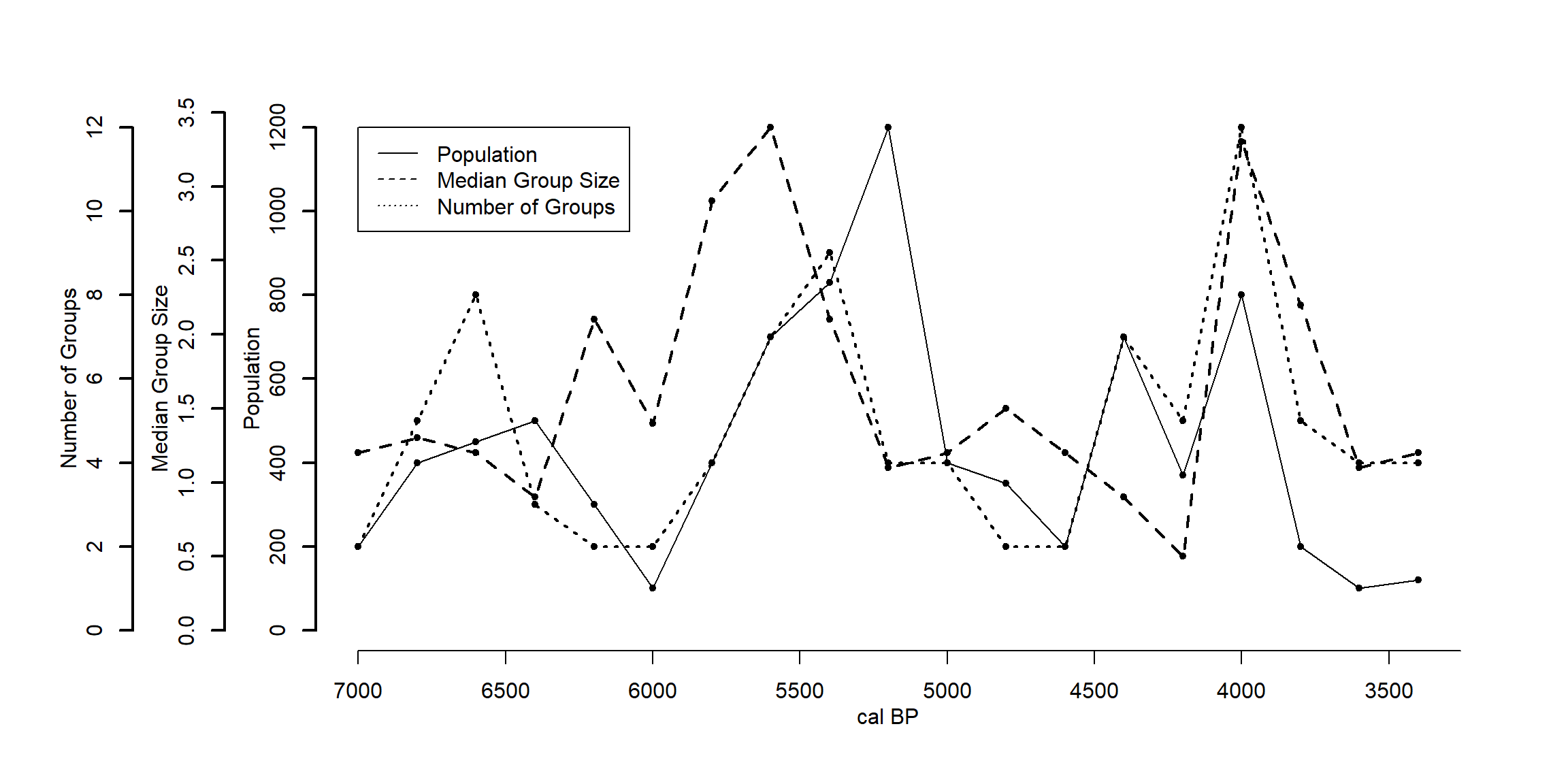
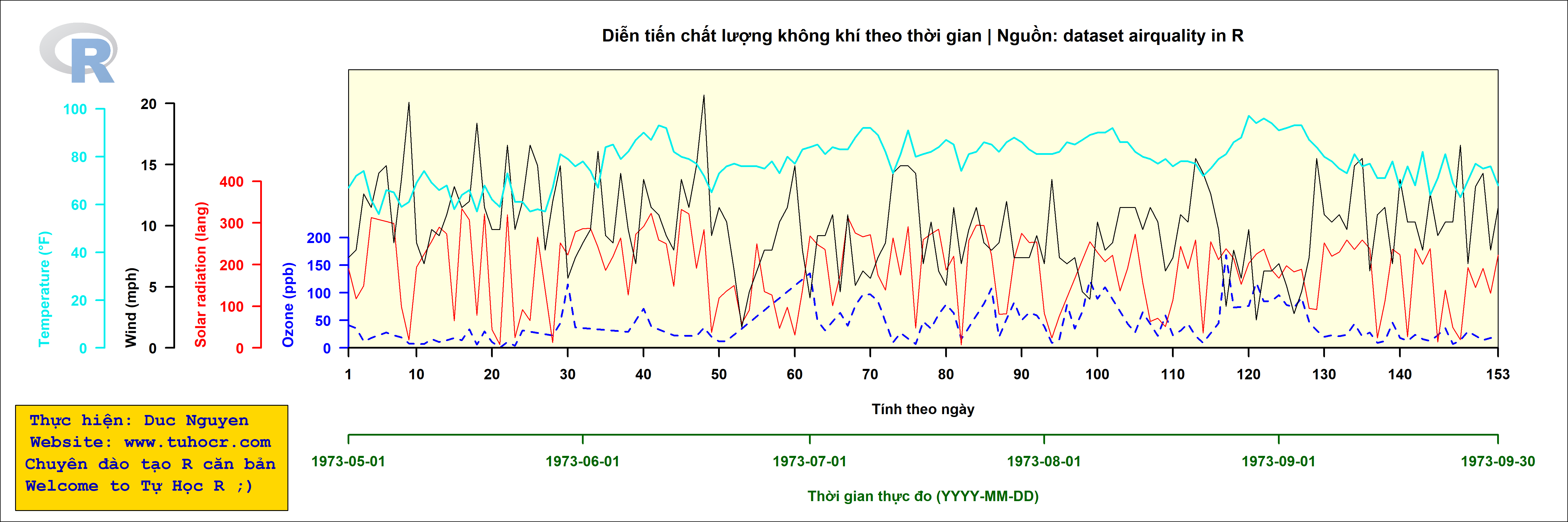
airquality -> df

df$year <- 1973

df$date <- paste0(df$year, "-", df$Month, "-", df$Day)

df$date <- as.Date(df$date)

df$time <- row.names(df)

df$time <- as.numeric(df$time)

# options(max.print = 100000)

# windows(width = 18, height = 6) # vẽ chuẩn trên này

# save chuẩn, nếu không khớp cần chỉnh trực tiếp lại
png(width = 18,
    height = 6,
    units = "in",
    res = 300,
    filename = "do_thi_nhieu_truc_tung.png")

# oldpar <- par(no.readonly = TRUE)

par(oma = c(0, 0, 0, 0))

par(mar = c(10, 20, 4, 4))

par(xpd = TRUE)

# par(bg = "aliceblue")

plot(formula = Ozone ~ time, 
     data = na.omit(df[, c("Ozone", "time")]), # nối liền NA
     axes = FALSE, 
     ylim = c(0, max(df$Ozone, na.rm = TRUE)*3),
     xaxs = "i",
     yaxs = "i",
     xaxt = "n",
     yaxt = "n",
     xlab = "",
     ylab = "",
     lty = 2,
     lwd = 2,
     type = "l",
     col = "blue", 
     main = "",
     xlim = c(1, max(df$time))
)

# Change the plot region color
rect(par("usr")[1], par("usr")[3],
     par("usr")[2], par("usr")[4],
     col = "lightyellow") # Color

###

par(new = TRUE)

plot(formula = Ozone ~ time, 
     data = na.omit(df[, c("Ozone", "time")]), # nối liền NA
     axes = FALSE, 
     ylim = c(0, max(df$Ozone, na.rm = TRUE)*3),
     xaxs = "i",
     yaxs = "i",
     xaxt = "n",
     yaxt = "n",
     xlab = "",
     ylab = "",
     lty = 2,
     lwd = 2,
     type = "l",
     col = "blue", 
     main = "",
     xlim = c(1, max(df$time))
     )

box(which = "plot")
box(which = "figure")
box(which = "inner")
box(which = "outer")

# points(formula = Ozone ~ time, 
#        data = na.omit(df[, c("Ozone", "time")]), 
#        pch = 20, 
#        col = "black")

## trục Y1

axis(side = 2, 
     # ylim = c(0, max(df$Ozone, na.rm = TRUE)*3),
     at = c(0, 50, 100, 150, 200),
     labels = c(0, 50, 100, 150, 200),
     col = "blue",
     col.axis = "blue",
     font = 2,
     lwd = 2,
     las = 2)

mtext(side = 2,
      text = "Ozone (ppb)",
      line = 3,
      font = 2,
      col = "blue",
      adj = 0)

## trục X1

# axis(side = 1,
#      at = pretty(range(df$time), 10) # tự chia khoảng cho hợp lý
#      )

## scale X1

time_1 <- c(1, 10, 20, 30, 40, 50,
            60, 70, 80, 90, 100, 110,
            120, 130, 140, 153)

axis(side = 1,
     at = time_1,
     labels = time_1,
     font = 2,
     lwd = 2
)

mtext(side = 1,
      text = "Tính theo ngày",
      line = 3,
      font = 2)

###

par(new = TRUE)

plot(formula = Ozone ~ date, 
     data = na.omit(df[, c("Ozone", "date")]), # nối liền NA
     axes = FALSE,
     ylim = c(0, max(df$Ozone, na.rm = TRUE)),
     xaxs = "i",
     yaxs = "i",
     xaxt = "n",
     yaxt = "n",
     xlab = "",
     ylab = "",
     type = "n",
     col = "black", 
     main = ""
)

## scale X2 (vì là datetime nên phải plot riêng cái mới,
# do R vẽ datetime theo numeric tính từ 1970-01-01)

axis(side = 1,
     at = c(seq.Date(from = df$date[1], to = df$date[153], by = "months"), df$date[153]),
     line = 5,
     labels = c(seq.Date(from = df$date[1], to = df$date[153], by = "months"), df$date[153]),
     font = 2,
     lwd = 2,
     col = "darkgreen",
     col.axis = "darkgreen",
)

mtext(side = 1,
      text = "Thời gian thực đo (YYYY-MM-DD)",
      line = 8,
      col = "darkgreen",
      font = 2)

### VẼ TRỤC Y2

par(new = TRUE)

plot(formula = Solar.R ~ time, 
     data = na.omit(df[, c("Solar.R", "time")]), # nối liền NA
     axes = FALSE, 
     ylim = c(0, max(df$Solar.R, na.rm = TRUE)*2),
     xaxs = "i",
     yaxs = "i",
     xaxt = "n",
     yaxt = "n",
     xlab = "",
     ylab = "",
     type = "l",
     col = "red", 
     main = "",
     xlim = c(1, max(df$time))
)

## trục Y2

axis(side = 2, 
     # ylim = c(0, max(df$Solar.R, na.rm = TRUE)*2),
     at = c(0, 100, 200, 300, 400),
     labels = c(0, 100, 200, 300, 400),
     col = "red",
     col.axis = "red",
     font = 2,
     lwd = 2,
     las = 2,
     line = 5)

mtext(side = 2,
      text = "Solar radiation (lang)",
      line = 8,
      font = 2,
      col = "red",
      adj = 0)


### VẼ TRỤC Y3

par(new = TRUE)

plot(formula = Wind ~ time, 
     data = na.omit(df[, c("Wind", "time")]), # nối liền NA
     axes = FALSE, 
     ylim = c(0, max(df$Wind, na.rm = TRUE)*1.1),
     xaxs = "i",
     yaxs = "i",
     xaxt = "n",
     yaxt = "n",
     xlab = "",
     ylab = "",
     type = "l",
     col = "black", 
     lwd = 1,
     lty = 1,
     main = "",
     xlim = c(1, max(df$time))
)

## trục Y3

axis(side = 2, 
     ylim = c(0, max(df$Wind, na.rm = TRUE)*1.1),
     col = "black",
     col.axis = "black",
     font = 2,
     lwd = 2,
     las = 2,
     line = 10)

mtext(side = 2,
      text = "Wind (mph)",
      line = 12,
      font = 2,
      adj = 0,
      col = "black")

### VẼ TRỤC Y4

par(new = TRUE)

plot(formula = Temp ~ time, 
     data = na.omit(df[, c("Temp", "time")]), # nối liền NA
     axes = FALSE, 
     ylim = c(0, max(df$Temp, na.rm = TRUE)*1.2),
     xaxs = "i",
     yaxs = "i",
     xaxt = "n",
     yaxt = "n",
     xlab = "",
     ylab = "",
     type = "l",
     lwd = 2,
     lty = 1,
     col = "cyan2", 
     main = "",
     xlim = c(1, max(df$time))
)

## trục Y4

axis(side = 2, 
     ylim = c(0, max(df$Temp, na.rm = TRUE)*1.2),
     col = "cyan2",
     col.axis = "cyan2",
     font = 2,
     lwd = 2,
     las = 2,
     line = 14)

mtext(side = 2,
      text = "Temperature (\u00B0F)",
      line = 17,
      font = 2,
      adj = 0,
      col = "cyan2")

title(main = "Diễn tiến chất lượng không khí theo thời gian | Nguồn: dataset airquality in R")

###
library(png)
library(grid)
logor <- readPNG("logor.png")
grid.raster(logor, x = 0.05, y = 0.9, width = 0.05)

###
library(unikn)
library(showtext)

par(lheight = 1.15)

###
# https://cran.r-project.org/web/packages/unikn/vignettes/text.html

mark_v1 <- function (labels, x = 0, y = 0.55, x_layout = NA, y_layout = "even", 
                     col = "black", col_bg = Seeblau, cex = 2, font = 2, new_plot = "none", ...) 
{
  if (new_plot == FALSE || tolower(new_plot) == "false" || 
      substr(tolower(new_plot), 1, 2) == "no") {
    new_plot <- "none"
  }
  unikn:::plot_text(labels = labels, x = x, y = y, x_layout = x_layout, 
                    y_layout = y_layout, col = col, col_bg = col_bg, cex = cex, 
                    font = font, new_plot = new_plot, col_bg_border = NA, 
                    pos = 4, mark = TRUE, ...)
}
###

rect(-43, -68,
     -7, -24,
     col = "gold") # Color

mark_v1(labels = c("Thực hiện: Duc Nguyen", 
                   "Website: www.tuhocr.com", 
                   "Chuyên đào tạo R căn bản", 
                   "Welcome to Tự Học R ;)"), 
     x = -40, 
     y = -30,
     family = "mono",
     y_layout = "flush",
     col_bg = "transparent",
     col = "#0000b3",
     cex = 1.2)

# par(oldpar)

dev.off()

knitr::include_graphics("do_thi_nhieu_truc_tung.png") 

Full-size: https://thongkesinhhoc.com/do_thi_nhieu_truc_tung.png